Stereoscopic Depth Sensing – A Python Approach

*All images used here are a property of http://vision.middlebury.edu/stereo

BRIEF INTRODUCTION TO DEPTH SENSING:

The human eye is truly an amazing piece of technology (if you look at it from a technology perspective); the things it is capable of achieving is truly amazing. Of the multitude of its capabilities, one very special capability which most single lens camera are unable to mimic, is the capability to perceive objects by their closeness with respect the camera. Lets say you have an image like this:

A generic image to describe the concept of depth sensing

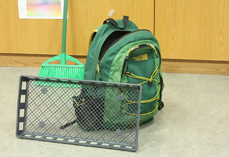
We, as humans, are easily capable of determining that the mesh-tray is closest to us, then the backpack; behind it is the broomstick and beyond that, the background.

So, we are easily capable of breaking down the image into 4 layers:

• Layer 1 : Mesh Tray (closest)
• Layer 2 : Backpack
• Layer 3 : Broomstick
• Layer 4 : Background

This happens because, we see with both our eyes. If you ever notice, any scene you see with only your right eye, appears to be a bit shifted when seen from the left eye. This shift in the position of objects due to our stereo vision (binocular vision) depends on how far the object is from us. The closer it is, the more is gets shifted; the farther it is, the less the shift. And this is what gives rise to our capacity to sense depth in front of us.

The objective here is to write an algorithm capable of processing depth from stereo image pairs. Simply put, a trial to mimic our brain’s response to our vision, that allows us to perceive depth.

In this diary, a few technical references are made. I will explain them here itself.

• Stereoscopic Images : Images taken using a camera with 2 lenses on the same horizontal level, but placed at a certain separation. The images taken are quite equivalent to how we see, binocular vision.
• SAD : Sum of Added Differences. When the values of 2 matrices are subtracted to form a new matrix, and all the elements are added together to form a single scalar value.
• Image Pyramids : The same image (the one being processed) is taken in various sizes and processed separately. A median from all the processed images finally gives the output.
• RGB : Red – Green – Blue image. Standard format of coloured images.

The updates will be made in the form of logs. I will be progressing on the code as I update here, so this might not finish off in one go.

---

---

---

LOG UPDATE 1 : [24/05/2017 – 0947 hrs]

Starting on a new project. I will be keeping logs here on the updates. The project is related to the sensing of depth of objects in stereoscopic image pairs.

The steps to the algorithm are roughly sketched as:

1. Reading pixel data from image
2. Convert image to Edge-only Image for Stereo-image pair
3. Comparing data between edge -highlighted stereo images
4. Implement a sub-pixel accuracy approach

Further additions to be made if the output is not up to the standard.

Signing off for now. Ciao.

---

---

LOG UPDATE 2 : [26/05/2017 – 1656 hrs]

Started working on the stereo image sets. Since, these are RGB images, they need to be converted to Grayscale to reduce complexity during further processing.

There are 2 ways to achieve RGB-to-Grayscale conversion:

• Unweighted: In this case, we simply take an average of the red, green, blue pixel data. There is no biasing and is not related to human vision.
  We can consider it like this:

pixel [gray] = ( pixel [red] + pixel [green] + pixel [blue] ) / 3

• Weighted: In this case, we take into account, the visibility factor of different colors to the human eye, and accordingly, set a bias to the average.
  We can consider it like this:

pixel [gray] = ( pixel [red]*0.299 + pixel [green]*0.587 + pixel [blue]*0.144 )

The differences seem quite trivial to the human eye. Hoping, it will make some difference in the final computation.

Need to proceed on the tile breakdown of the image next. Will be updating soon.

Adios.

---

---

LOG UPDATE 3.1 : [28/05/2017 – 0057 hrs]

Okay, I won’t deny; this is getting pretty tiring. Have been coding for sometime now, and finally found a feasible way of generating a window from the image. The dimensions of the windows are generated automatically, as a function of the actual length and height of the original image. Generating a window from the image isn’t really the big deal here, what we need to account for is the way in which, we can call it from a nested loop without generating any exceptions.

Okay, I guess I shouldn’t be cryptic anymore. So, what the hell is this window? The window here is a slice of the image which we can slide along another image to compare a similar such window there. I hope you’re getting a vague picture of what I am aiming to do. Yes, the aim is to check for the most similar block on the other image, and then find the distance between these 2 blocks.

Here is an image of the window getting generated from the right stereo image. In this project, the comparison will be made of the right image to the left one.

 

Colored Image Window

Grayscale Image Window

It seems Log Update 3 will continue for a while…

Got to get some rest now. Will be writing up the comparison algorithm tomorrow, if things go well.

---

---

LOG UPDATE 3.2 : [31/05/2017 – 1203 hrs]

Okay. So, the basic block matching is done now. I will give you a brief understanding of what I have covered in this section.

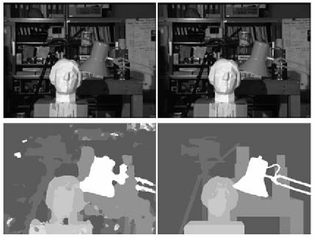
The idea of stereoscopic image pair is the image of the same scene taken side by side, which  generates a shift of objects based on their proximity to the viewing element. This image here will show you what stereoscopic really means.

 

Left Sterescopic Image

Right Stereoscopic Image

These 2 images on overlaying on each other generates this image:

Stereoscopic Image Pairs overlaid on each other to highlight the disparity.

Hence, the objective is to do the following:

• Break the Right Image into blocks of a given specific dimension (keeping in mind that no out-of-bounds exception occur)
• Break the Left Image into blocks ina similar manner
• Set a range of pixels within which, the comparison for matching block will be done.
• Select a block from Right Image and run that through the pixel range on the Left Image.
• On finding the closest value (calculating Sum of Added Differences should be least), setting that on a null image.
• Continue for all the blocks on the Right Image

In Python, images are represented as 2-D arrays which we can manipulate as per our need. Hence, the first thing to be done after slicing the images, is to check for the closest matching block on the other image.

This image will well illustrate what is being intended here:

Selected Block from Right Image

Let us consider that the green tile is the block we are considering for matching. Next we take a portion from the other image (Left Image in this case) and slide along a window in the same row to find closest matching block. We break the portion into blocks of equal sizes and check each block for the closest match by comparing to the source block from the Right Image. The below image will better illustrate this:

The Red block represent the same position as the block on Source image.
The Green block represents the closest matching block on Left image.

Now, the Sum of Added Differences (SAD) is the means of finding the disparity. Since, the images are represented as 2-D arrays, any block of (m x n) pixels will have an (m x n) array associated to it. If all the pixels are a perfect match, then all the color values associated to each pixel will be exactly the same. Hence, the 2  blocks will be identical. But, such identical pairs don’t occur in stereo pairs and we need to look for the block which has the closest match. Now, this will show you how to calculate the SAD.

Hence, it is understandable, that as the SAD value decreases, the closer the matches become.

The positions for which we get the least SAD values are recorded and, we get a optimum disparity value as:

disparity =
position of selected Right block – position of closest matching Left block

What we do with this disparity value that we find is very simple. We take an an empty image with dimensions equal to that of the source image. Now, we populate the image block wise (consider block size is m x n). Let us say we take one block at (15,15). We find that, the closest matching block is at (15, 38). Hence, the disparity value will be 23. This 23 will be populated in a empty block (m x n) and then added to the position (15,15) on a null image.

Doing this for the whole image generates a rough disparity map.

I will show you how far I have reached with my code:

The outcome of simple block matching algorithm on stereo images

As can be seen, a basic depth map has been visualised. But, a lot of noise has crept in as well. It seems, there is a need to resort to additional processes for better approximations. This might take a while to get around to.

Lots of work needs to go into this. See you until next time.

---

---

LOG UPDATE 4 : [06/06/2017 – 0003 hrs]

So, a minor upgrade to the code. Till now, what I worked on simply mapped the disparity, based on the best matching block. On sliding the block and finding the SAD value, we chose the block with the least SAD and the distance between the position of that block on the right image and the position on the left image is considered the disparity value.

But, what if, the blocks did not map perfectly in both images. Let us consider a scenario in which the matching block start in between 2 consecutive pixel. Although this is a very minor issue, it still needs to be resolved and there is an extremely graceful way to tackle such a problem. We need to resort to interpolation.

The SAD – disparity plot. The plot generates a parabola for 3 consecutive points.

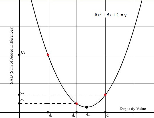
d₂ is the disparity of the best matching block and C₃ is the corresponding SAD value of d₂ block, d₁ is the block just before d₂ with SAD value C₁, d₃ is the block just after d₂ with SAD value C₂.
As you can see, d₂ may not be the minimum value of disparity. We can understand that the minima of this parabola is the true minimum value of disparity. We assign the name d_est to this true minimum. The way to calculate this is called Lagrangian Interpolation.

A brief derivation of this formula is given in the link underneath:

Lagrange Interpolation

On implementing this sub-pixel accuracy algorithm in the existing code, very minor changes were visible (primarily on low-resolution images). Since, there were no major improvements for the test image, I am not providing any progress-report output. The output given here is just that of the test image post subpixel accuracy implementation:

The outcome of block matching algorithm with subpixel accuracy on stereo images

I hope to start working on smoothing of these disparity maps soon. See you soon.

---

---

LOG UPDATE 5 : [09/08/2017 – 1110 hrs]

Its been a while since I updated things here, but that because I was stuck; really stuck and I couldn’t find a way out. There was no further enhancements and changing block sizes and iterator ranges did not enhance the depth map. So, I took a break.

Cutting through the chase, I finally stumbled upon a means to enhance the outcomes and it simply came out of the blue. I was checking up some other functions and operations, and decided to write a code for edge detection using the Prewitt Operator. I intend to make another post regarding the edge detection techniques soon. But, for now, lets just focus on the idea of how the outcome was enhanced.

So, the first thing that hit me was that, in stead of generating blocks using every pixel’s RGB data, how would it work if we could work only on features. So, once the edges are highlighted and every other portion is dark, the computational complexity would also reduce, since the data was mostly 0 for black regions.

So after applying the Prewitt operator on both the left and right images, this is the output:

 

Left Image with Highlighted Edges

Right Image with Highlighted Edges

The block matching algorithm is then applied on this stereoscopic image pair. The process of block matching is same as before.

With these modifications applied, the outcome came up as this:

Disparity Map Generated from Edge Highlighted Stereo-images

---

---

This looks really impressive on the whole but when tested on another image set, the output image came out with some discrepancies. This image pair has a lot of uni-colour section in the image after the edges have been highlighted.

 

Left Image

Right Image

As you can see, this image has a lot of white (uni-colour) and on generation of the edge-highlighted image, both images might have disparity, but due to the color tone being same, not detect it.

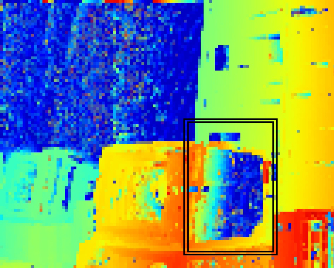
Using the process of edge detection, we got this stereo output leading to a disparity map as shown below:

 

Left Image (Post-processing)

Right Image (Post-processing)

---

---

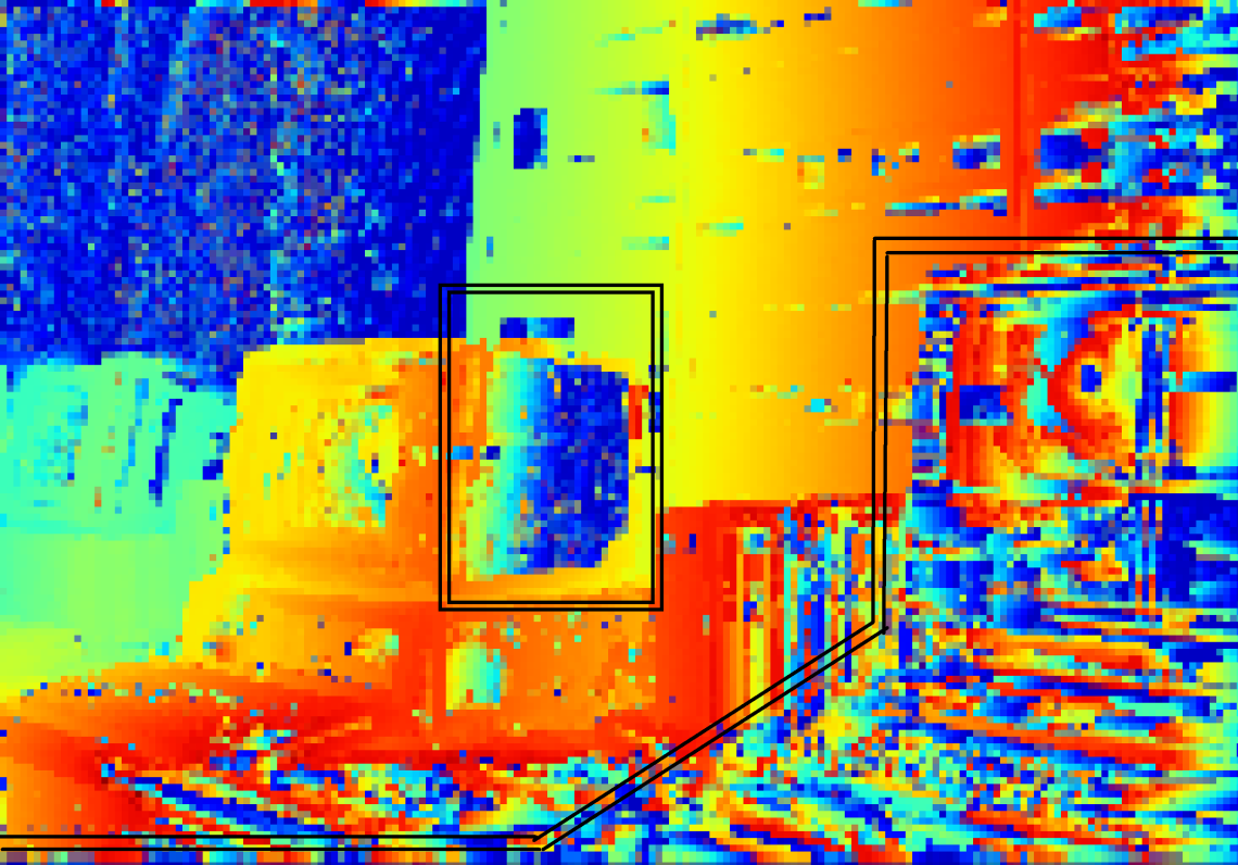As is visible, irrespective of the low resolution, the highlighted regions have discrepancies. The boxed regions need to have a warmer colour (in the range of yellow and orange) and the monitor in the front needs to be redder. But they come up in shades of blue. Need to look into that.

Feels good to be back. Will catch you next time with an apt resolution to this issue.

---

---

LOG UPDATE 5 : [04/09/2017 – 2338 hrs]

Okay, so I have reached the final leg of this project and am about to give you the final details. Additionally, I will also update all project details in my Github and put in the link here.

So, the errors we faced previously were mainly due to 2 problems.

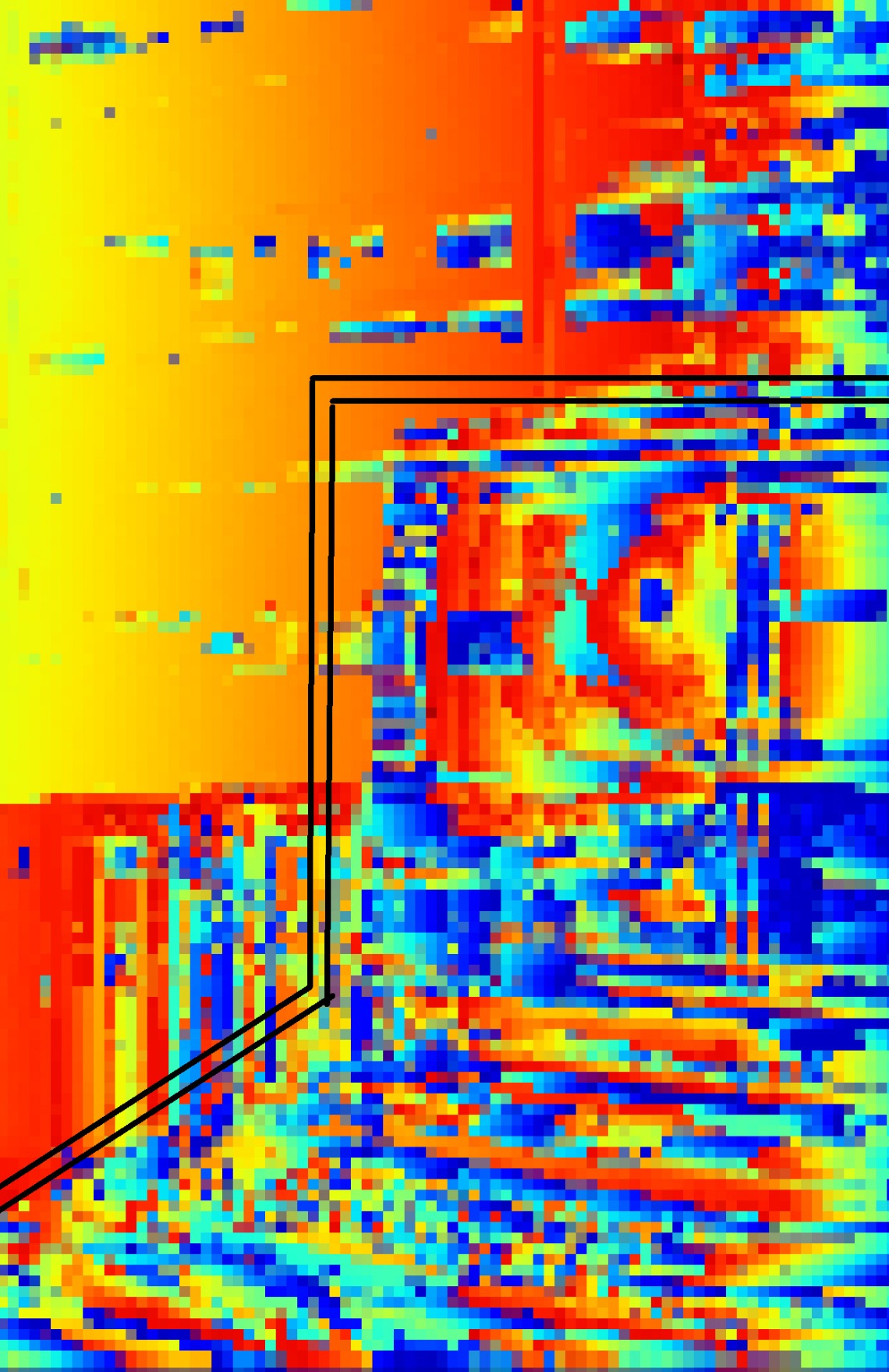
The first issue was with this portion of the image:

Disparity Map Error 1

Even though, the section was closer than the disparity shows, it was not detected properly. This as I found out, was due to using only the edge-detected image (edge map as I refer to it). Since, there was a uniform colour here, the detection found the disparity to be very close due to the uniformity. Hence, it was rectified by using a mixing the edge map and the source image with a varying degree of opacity on either.

On mixing them, the image for disparity checking came up as this:

 

New Left Image

New Right Image

The second issue, after much testing was with the span in which the disparity was being checked.

Disparity Map Error 2

Now, since the map was unable to find the perfect match, it chose to stay with the closest matching block which happened to be the neighboring blocks. Increasing the search span rectified this problem. So, the solutions were primarily:

• Mix the colour image to the edge map and then use those as the stereoscopic image pair.
• Increase the search span in case of discrepancy at higher disparity ranges.

After introducing the two rectifications, the outcome came up as this:

 

Left Image

Right Image

Final Rectified Disparity Map

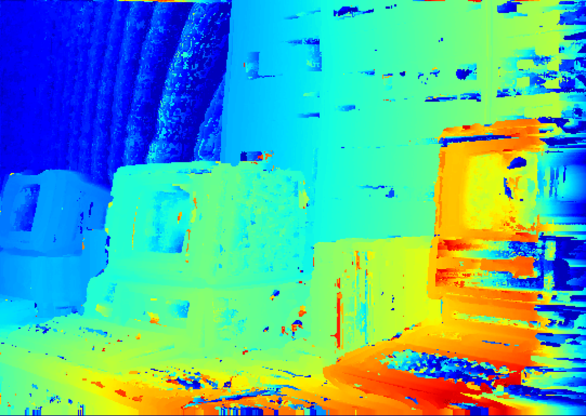
As you can see, the depth map seems to be showing the outcome as expected.

---

---

LOG UPDATE 5 : [05/09/2017 – 0026 hrs]

The final update in this project.

The objective was to generate a 3D map of the environement from 2 stereoscopic images.

So, this final section introduces the idea of how to generate a 3D environment render from a disparity map.

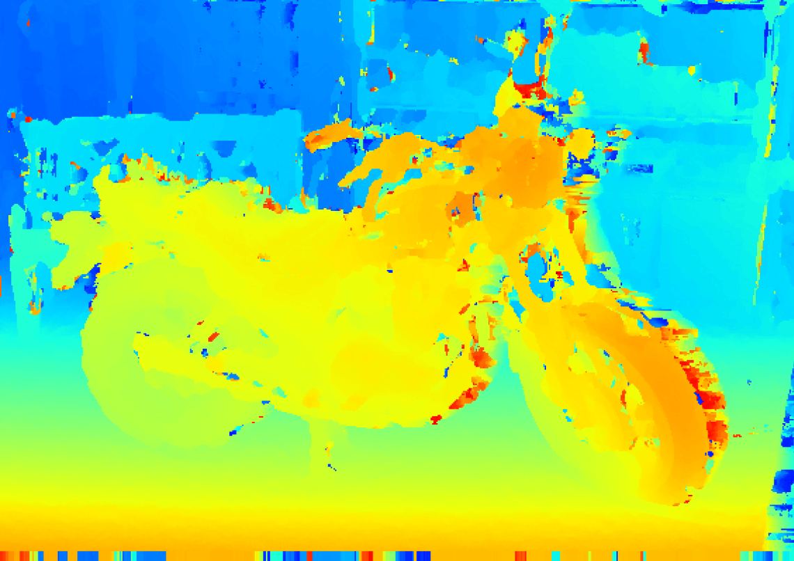
Let us take this disparity map:

So, as the disparity value rises, the colour warmth rises proportionally. Now, to explain how to do a 3-D plot, lets say the X and Y axis simply represent the height and width of the image. So, each (x,y) combination will represent each pixel on the image. Each pixel in the disparity map represents the disparity which is basically a numeric representation of how close that pixel is to the camera.

These 2 images will further clarify what I am saying here:

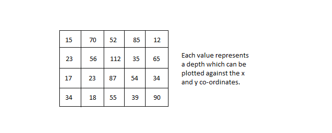
The depth values are actually the data generating the original disparity map. Now, this image will help understand how to use the depth data to map a 3-D plot of the environment.

Mapping the disparity map in 3 dimensions

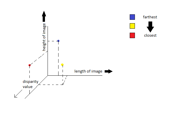
The depth details are finally plotted in the z-axis and plotted against the X and Y co-ordinates.

After finally generating the plot, this is the video generated by stitching images taken from every angle.

---

---

There you go, that’s the end of the depth mapping project.

Signing off.

GitHub Repos – 3D Stereo Render